Imaginative Consultancy in Computational Fluid Dynamics

Computational Fluid Dynamics Worked Examples

All the problems are extracted from our publication "Computational Fluid Dynamics Recipes - Outline & Worked Examples" and all formulae references are from the book. To order our publications, please visit our page here.

We will add more and more problems as we go on.

To support this effort, please either order our publications or ask you library to do so.

One Dimensional Heat Conduction without a source

Example 8.1 - 1D Heat Conduction without a source

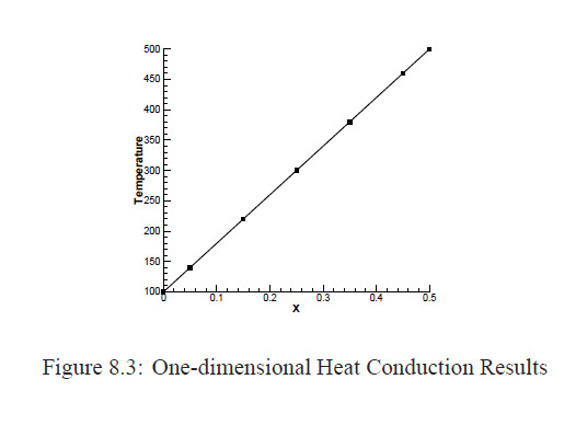
Consider heat conduction in an insulated bar whose ends are kept at constant temperature, as shown in Figure 8.1. Solve the heat conduction equation and find the temperature distribution in the bar. Data: T _wb = 100^◦C, Teb = 500^◦C, κ = 1000 W/m.K, A = 0.001 m2, L = 0.5 m

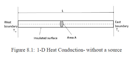
Since heat can only be transfered through the ends of the bar, this is a onedimensional problem along the xaxis.

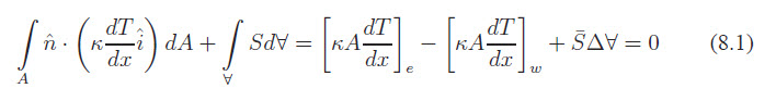
Integral equations

The integral equations for a typical control volume can be written in accordance with Eqn.(7.4). Bearing in mind that here we have φ = T and Γ = κ, we may write

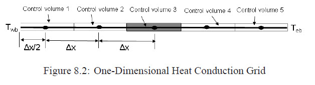
The Grid

We use an equally spaced grid, that is a uniform grid, in a way that the east face of the first control volume is on the east boundary and the west face on the west boundary. The spatial increment Δx has been chosen such that the number of control volumes are exact multiplier of the length of the bar. Of course any other arrangement can be used as long as you are consistent in your formulation.

Discretization

In discretizing Eqn.(8.1), we need to distinguish between the inner cells and boundary cells.

1. Inner Nodes: defined by

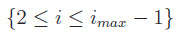
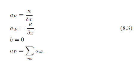
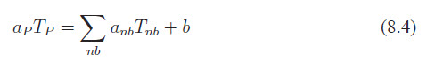
   For the inner cells we use the discretization of Eqn.(7.19) to write

   

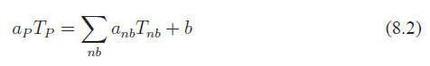
   where

   


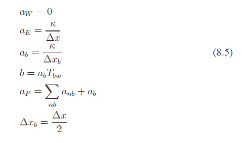
2. The west Node: defined by {i=1}

   Here, we have a Dirichlet boundary condition T_w = T_wb. Using Eqn.(7.34), we can write

   

   where

   


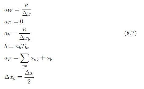
3. The east Node: defined by i=i_max

   This is similar to the west boundary and we can write

   

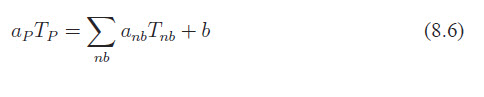
   where

   

System Solver

We use the GaussSeidel method of Section3.1.1 to solve these equations. The iteration converged after 24 steps for the allowed error of 0.0001. The temperature distribution is shown in Figure 8.3.

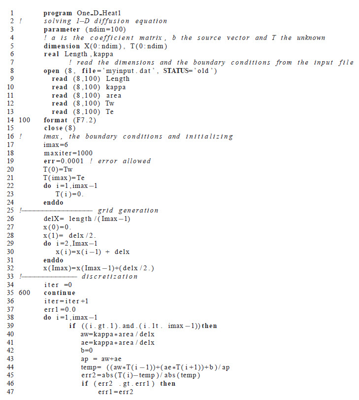
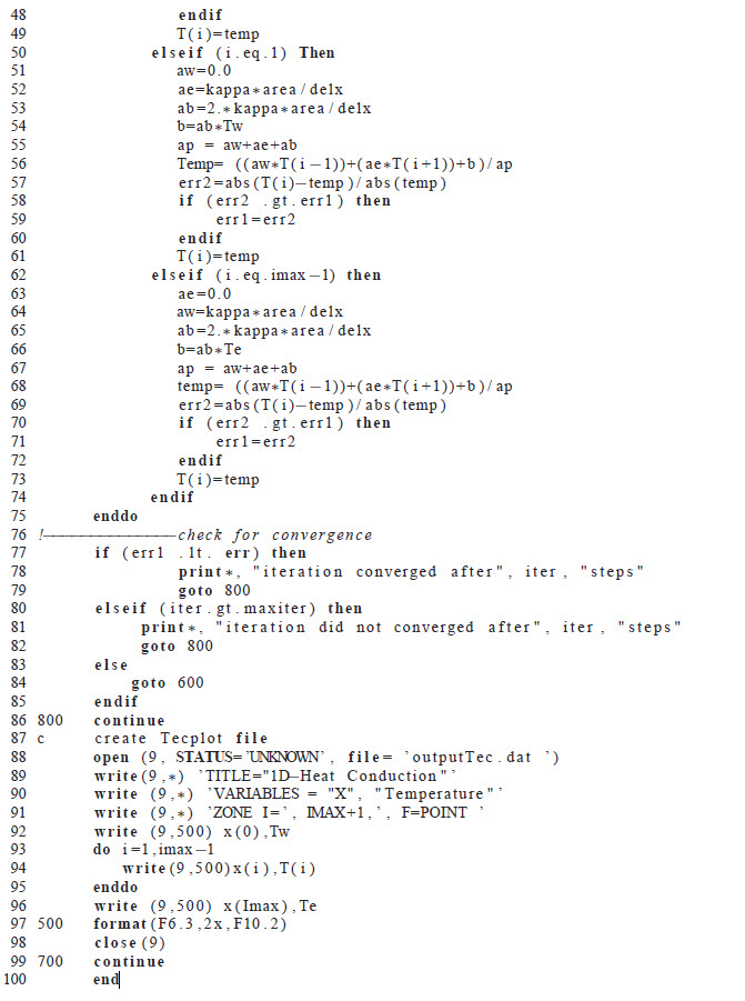
The Code