Imaginative Consultancy in Computational Fluid Dynamics

Computational Fluid Dynamics Worked Examples

All the problems are extracted from our publication "Computational Fluid Dynamics Recipes - Outline & Worked Examples" and all formulae references are from the book. To order our publications, please visit our page here.

We will add more and more problems as we go on.

To support this effort, please either order our publications or ask you library to do so.

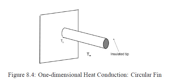
One Ddimensional Heat Cconduction: Circular Fin

Example 8.2 - 1D Heat Cconduction: Circular Fin

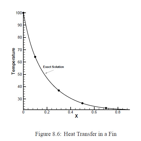
Consider a cylindrical fin with uniform crosssectional area A, shown in Figure 8.4. The base is at temperature of T_b and the tip is insulated. The fin is exposed to an ambient temperature of T_∞. Calculate the temperature distribution along the fin and compare the results with the analytical solution. Data : T_B = 100^◦C, T_∞ = 20^◦C, L = 1 m, Peclet Number=(Pe)=hP/(κA) = 25/m2 and κ is constant.

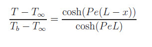
Heat is conducted along the fin and it is convected from the surface of the fin. The exact solution is given by

Integral Equation

The problem is in a steady state, that is, the same amount of the heat conducted from the base of the fin is removed from the fin by convection from the surface of it. Convection is given by the Newton’s law of convection

q=hP(T- T_∞)

where h is the convective heat transfer coefficient, P is the perimeter area of the fin, and T_∞ is the ambient temperature. Then we have

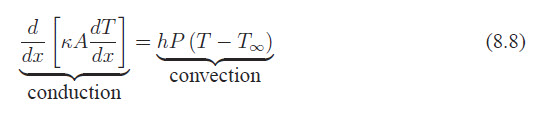
where κ is the thermal conductivity

Equation (8.8) is a onedimensional diffusion equation with a heat sink, which is a function of temperature at each node. From the mathematical point of view, we have a mixed boundary, as explained in Section7.4.3.

Since (κA) is constant, Eqn.(8.8) can be rewritten as

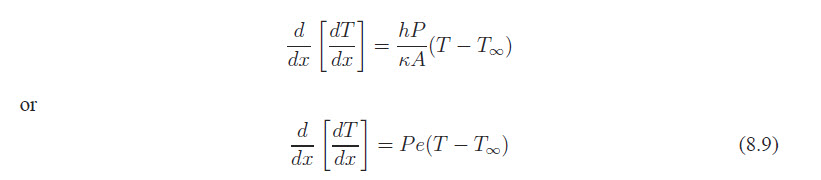
where Pe is the Peclet number.

Integrating this equation will result in

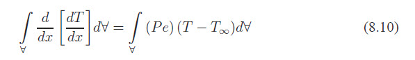
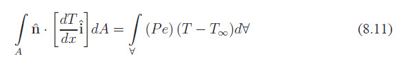
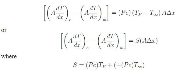
Using the Gauss’ theorem, Eqn.(1.6), we may rewrite Eqn.(8.10) as:

The Grid

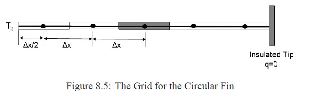
We could use a uniform grid with Δ x = 0.2m. The grid structure shown in Figure 8.5

Discretization

The discretization of the first integral in Eqn.(8.11) is similar to the previous Example. We should distinguish between three types of nodes (or control volumes): the inner nodes, the tip node (west boundary), and the base or the wall node (east boundary).

1. Inner nodes are defined by

   Since the fin is small in diameter, we have assumed that the fin’s surface temperature is the same as its center point P. Then, we can write

   

   With reference to Eqn.(7.7), we have

   

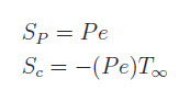
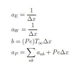
   Finally we can write

   

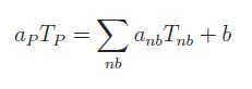
   where

   
2. Tip node is defined by {i = i_max}

   This tip is insulated. That is, we have

   

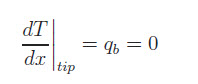
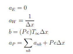
   This is a Neumann boundary condition. According to Eqn.(7.35), we can write

   

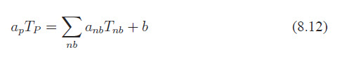
   where

   
3. Base node is defined by {i=1}

   Here, we have a Dirichlet boundary condition:

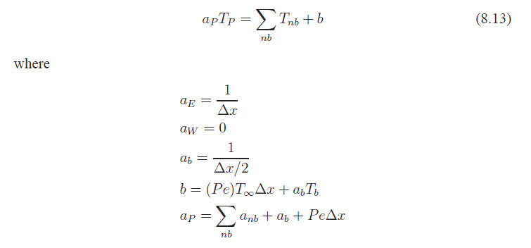
   T_w = T_(base) = T_b

   Using Eqn.(7.33), we can write

   

System Solver

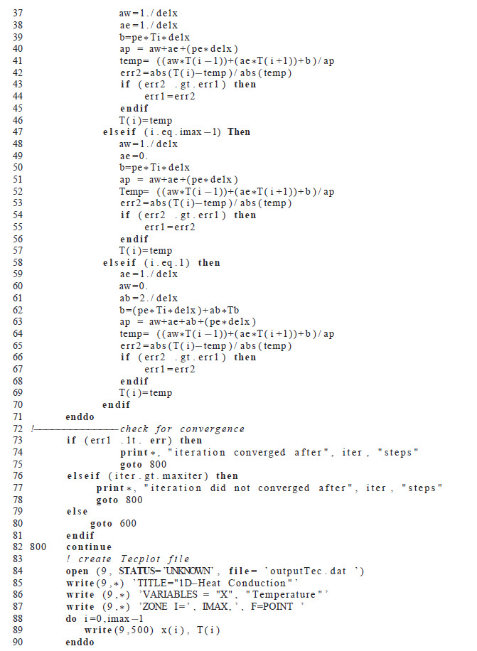
We use the Gauss-Seidel method of Section3.1.1 to solve these equations. The iteration converged after 10 steps for the allowed error of 0.0001. The temperature distribution is shown in Figure 8.3.

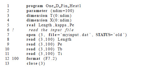
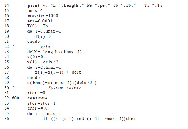
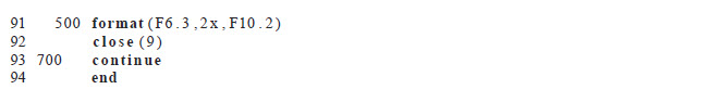
The Code