Imaginative Consultancy in Computational Fluid Dynamics

Computational Fluid Dynamics Worked Examples

All the problems are extracted from our publication "Computational Fluid Dynamics Recipes - Outline & Worked Examples" and all formulae references are from the book. To order our publications, please visit our page here.

We will add more and more problems as we go on.

To support this effort, please either order our publications or ask you library to do so.

Two Dimensional Heat Conduction

Example 8.3 - Two Dimensional Heat Conduction

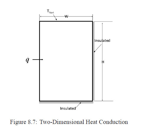
Consider a towdimensional thin plate of thickness t, height H and width W, shown in Figure 8.7. The west boundary receives a steady heat flux of q˙west and the south and the east boundaries are insulated. The north boundary is kept at TNorth. Find the steady state temperature distribution in this plate. Assume: t = 1.cm, κ = 1000W/mK, q˙W = 500kW/m2, T_north = 100^◦C, H = 0.4m and W =0.3m

Integral Equations

The integral equation for a two-dimensional problem is given by the Eqn.(7.22)

The Grid

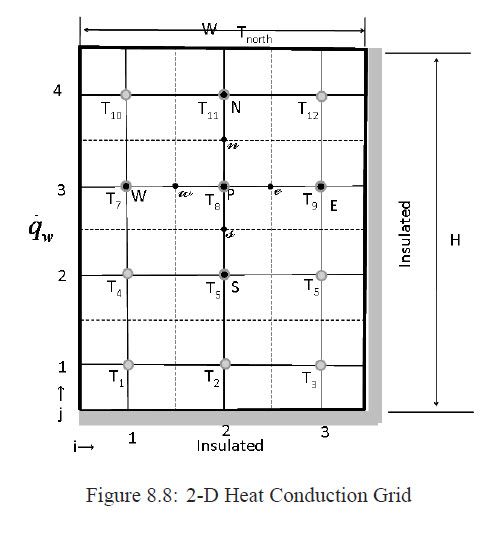
Assume a uniform grid with Δ x = Δ y = 0.1cm, where (i = 1 → imax and j = 1 → jmax) as shown in Figure 8.8.

Discretization

In this problem we have Neumann boundary conditions on three boundaries, west, east and south, and Dirichlet boundary condition on the north boundary. Furthermore, in addition to the distinction between the inner and boundary nodes, we need to distinct the corner cells. These cells have two faces exposed to the boundaries. The discretized equation in two dimensions is given by Eqn.(7.25).

1. Inner nodes: defined by {1 < i <i_max, 1 < j < j_max}

   The face areas are given by

   A_w = Δ y × thickness,

   A_e = Δ y × thickness,

   A_n = Δ x × thickness,

   A_s = Δ x × thickness

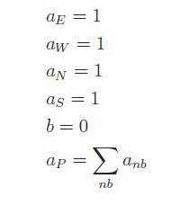
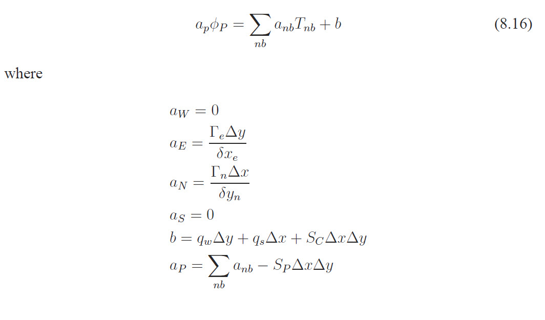
   Assuming i, j and k are zero at the origin, i = I_max and j = J_max at the north and east boundaries, and there are no heat sources or sinks, from Eqn.(7.25) we can write

   

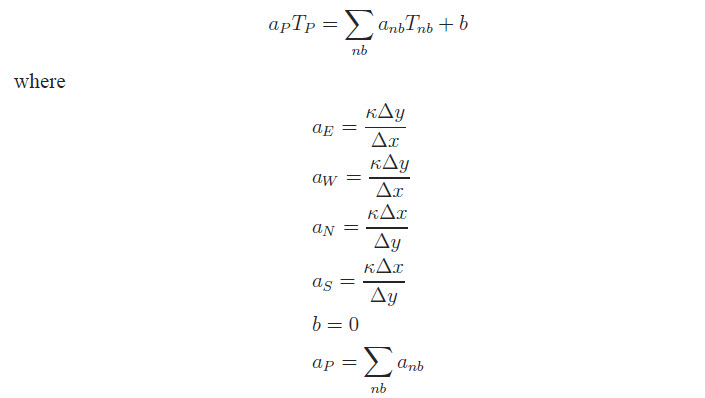
   With equal spacing (Δ x = Δ y) and constant thickness, if we multiply both side of the discretized equation by (Δ x / κ Δ y) , we will have

   
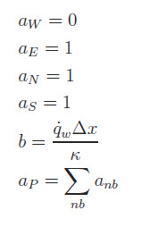
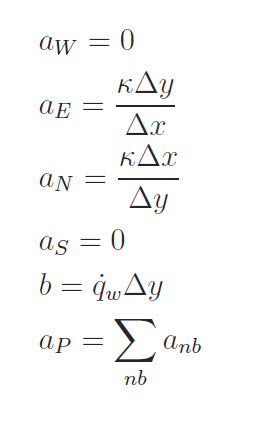
2. West boundary: defined by {i = 1, 1 < j < jmax}

   This boundary has a Neumann boundary condition with qb = q˙w. According to Eqn.(7.35) we have

   

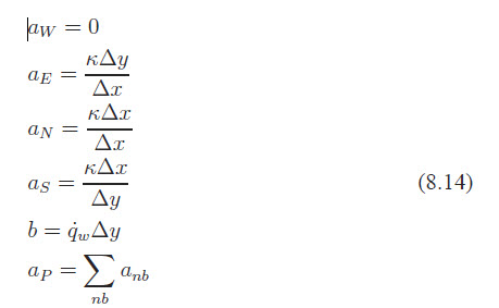
   Similar to the inner nodes, if we multiply all parameters by (Δ x / κ Δ y) , we get

   
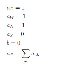
3. North boundary: defined by {1 < i < i_max, j = j_max}

   This boundary has a Dirichlet boundary condition. From Eqn.(7.34), we can write

   
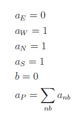
4. East boundary: defined by {i = i_max, 1 < j < j_max}

   This is another Neumann boundary condition with q_b = 0. According to Eqn.(7.35) we have

   
5. South boundary: defined by {1 < i < i_max, j = 1}

   Similar to the east boundary, we have

   
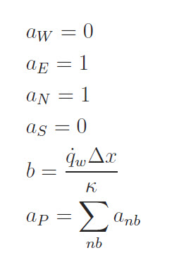
6. South-west corner (SW): defined by {i = 1, j = 1}

   The corner cells have boundary conditions acting on two of their faces. This particular control volume has a Neumann boundary conditions on its west and south faces. Let us assume the flux on the west boundary is q_w and on the south boundary is q_s, which is zero here. Then, following the argument for Eqn.(7.35), we can easily set up the discretized equation for SW corner cell as

   

   For the problem in hand we have q_w = q˙_w, q_s = 0 and S = 0. Therefore,

   

   or

   
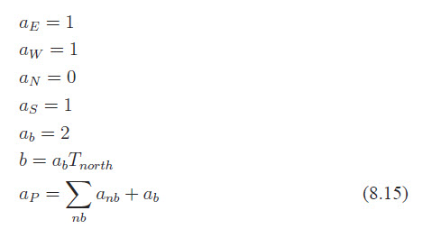
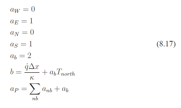
7. North-west corner (NW): defined by {i = 1, j = j_max}

   For this cell, we have a Neumann boundary on the west face and a Dirichlet boundary on the north side. Therefore we need to combine Eqns.7.34 and 7.35 to discretize the transport equation for this cell. Following the same procedures, we can write

   
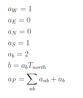
8. North-east corner (NE): defined by {i = i_max, j = j_max}

   This cell is similar to the NW corner and we can write

   
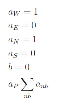
9. South-east corner (SE): defined by {i = i_max, j = 1}

   The control volume at the SE corner has a similar situation as the SW corner. Hence we can rewrite Eqn.(6) as

   

System Solver

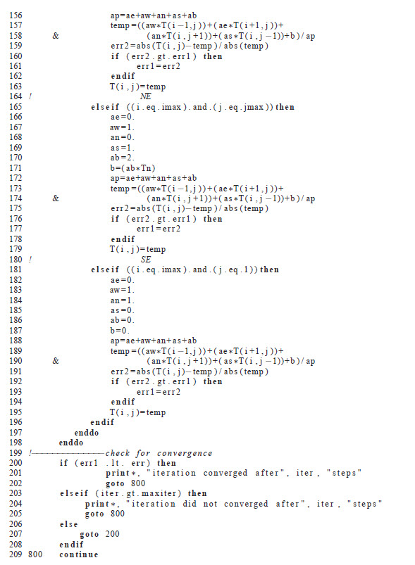
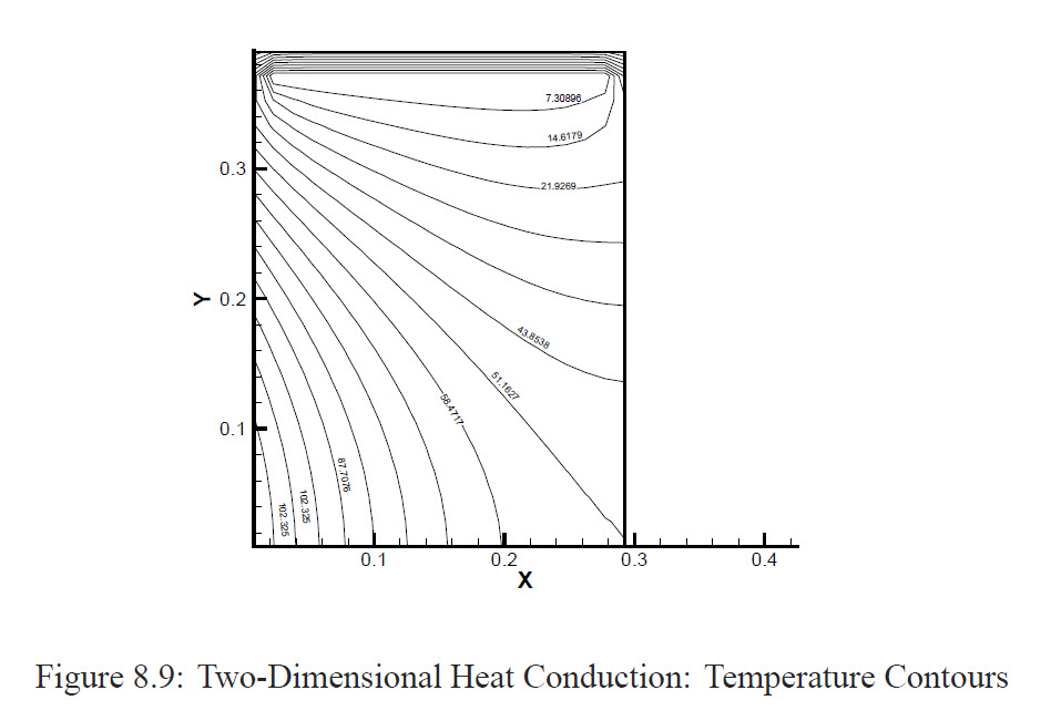
We use the Gauss-Seidel method of Section3.1.1 to solve these equations. Assuming I_max = 20, J_max = 21 and allowable error of 0.0001, the iteration converged after 1152 steps.

The contour plot of the temperature is shown in Figure 8.9.

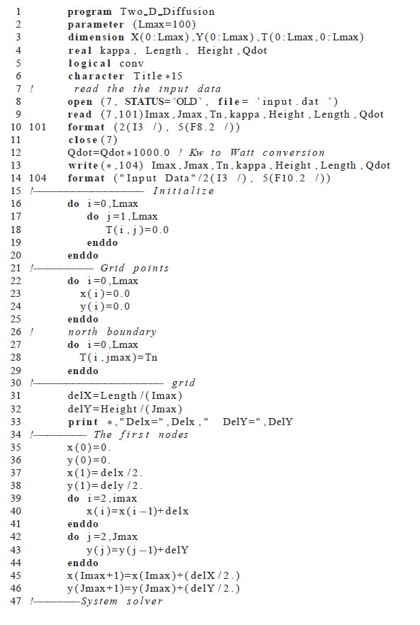
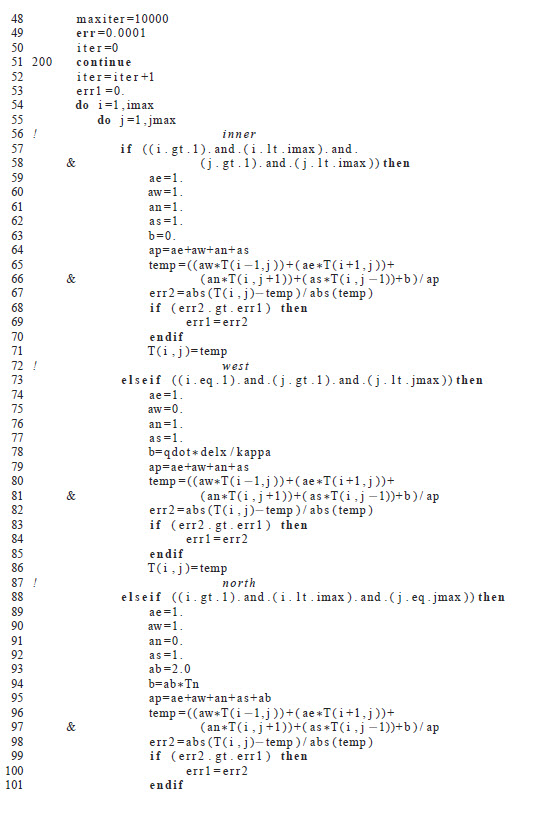
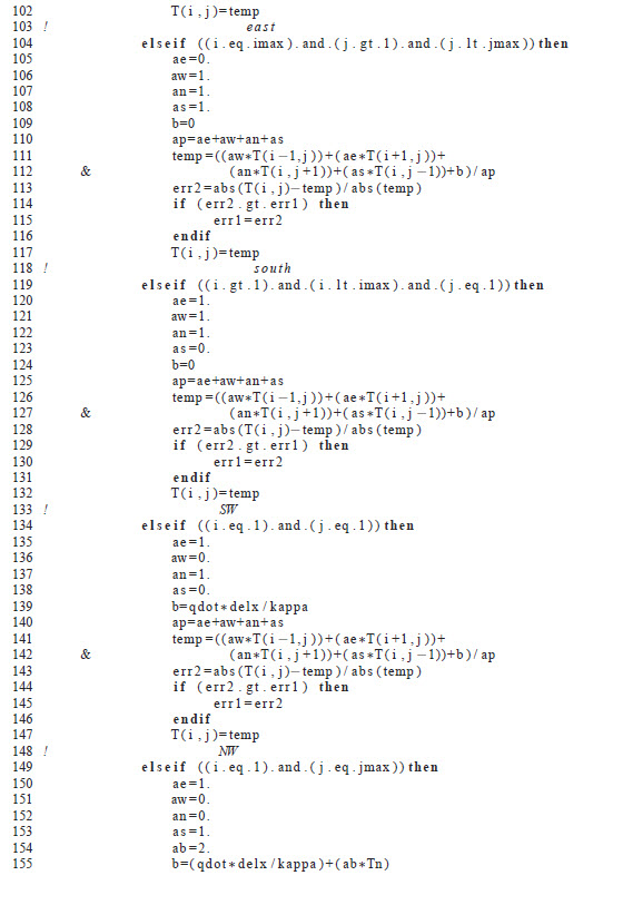
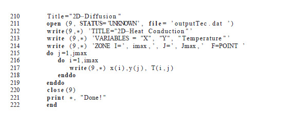
The code